Deep double descent explained (2/4) - Inductive bias of SGD

Inductive biases and the example of gradient descent.

\[\require{physics} \newcommand{\LL}{\mathcal{L}} \newcommand{\R}{\mathbb{R}} \newcommand{\D}{\mathcal{D}} \newcommand{\Dn}{\mathcal{D}_n} \DeclareMathOperator*{\argmin}{argmin}\]

Inductive biases

In the supervised learning problem, the model needs to generalize patterns observed in the training data to unseen situations. In that sense, the learning procedure has to use mechanisms similar to inductive reasoning. As there are generally many possible generalizable solutions, Mitchell (1980) advocated the need for inductive biases in learning generalization. Inductive biases are assumptions made in order to prioritized one solution over another both exhibiting the same performance on the training data. For example, a common inductive bias is the Occam’s razor principle stating that in case of equally good solutions the “simplest” one should be preferred. Another form of inductive bias is to incorporate some form of prior knowledge about the structure of the data, its generation process or to constrain the model to respect specific properties.

In the under-parameterized regime, regularization can be used for capacity control and is a form of inductive bias. One common choice is to search for small norm solutions, e.g. adding a penalty term, the $L_2$ norm of the weights vector. This is known as Tikhonov regularization in the linear regression setting (also known as Ridge regression in this case).

In the over-parameterized regime, as the complexity of $\mathcal{H}$ and the EMC increases, the number of interpolating solutions (i.e. achieving almost zero training error) increases, and the question of the selection of a particular element in $\text{argmin}_{h \in \mathcal{H}} L_n(h)$ is crucial. Inductive biases, explicit or implicit, are a way to find predictors that generalize well.

Explicit inductive biases

As illustrated in Belkin et al. (2019) , several common inductive biases can be used to observe a model-wise double descent (e.g. as the number of parameters $N$ increases).

Least Norm

For the model class of Random Fourier Features (defined in this post, by choosing explicitly the minimum norm linear regression in the feature space. This bias towards the choice of parameters of minimum norm is common to a lot of machine learning model. For example, the ridge regression induces a constraint on the $L_2$ norm of the solution, and the lasso regression on the $L_1$ norm. We can also see the support vector machine (SVM) as a way of inducing a least norm bias because maximizing the margin is equivalent to minimizing the norm of the parameter under the constraint that all points are well classified.

Model architecture

Another way of inducing a bias is by choosing a particular class of functions that we think is well suited for our problem. Battaglia et al. (2018) discuss different type of inductive bias considered by different type of neural network architectures. Working with images it is better to use a convolutional neural network (CNN) as it can induce translational equivariance, whereas the recurrent neural network (RNN) is better suited to capture long-term dependencies in a sequence data. Using a naive Bayes classifier is of great utility if we know that the features are independent, etc.

Ensembling

Random forest models use yet another type of inductive bias. By averaging potentially non-smooth interpolating trees, the interpolating solution has a higher degree of smoothness and generalizes better than any individual interpolating tree.

Implicit Bias of gradient descent

Gradient descent is a widely used optimization procedure in machine learning, and has been observed to converge on solutions that generalize surprisingly well, thanks to an implicit inductive bias.

We recall that the gradient descent update rule for parameter $w$ using a loss function $\LL$ is the following (where $\eta >0$ is the step size):

\[\begin{aligned} w_{k+1} = w_k - \eta \nabla \LL(w) \end{aligned}\]

Gradient descent in under-determined least squares problem

Consider a non-random dataset $\{(x_i, y_i)\}_{i=1}^n$, with $(x_i, y_i) \in \R^d\times\R$, for $i \in \{1, \dots ,n\}$ and let $\mathbf{X}\in \R^{n\times d}$ be the matrix which rows are the $x_i^T$ and $y \in \R^{n}$ the column vector which elements are the $y_i$. We consider the linear least squares:

\[\label{eqn:leastsquare} \min_{w\in \R^d} \LL(w) = \min_{w\in \R^d} \frac{1}{2}\norm{\mathbf{X} w - y}^2 \tag{1}\]

We will study the property of the solution found using gradient descent.

Definition 9 (Moore-Penrose pseudo-inverse). Let $\mathbf{A} \in \R^{ n\times d}$ be a matrix, the Moore-Penrose pseudo-inverse is the only matrix $\mathbf{A}^{+}$ satisfying the following properties:

$\mathbf{A} \mathbf{A}^+ \mathbf{A} = \mathbf{A}$ ,
$\mathbf{A}^+ \mathbf{A} \mathbf{A}^+ = \mathbf{A}^+$ ,
$(\mathbf{A}^+\mathbf{A})^T = \mathbf{A}^+\mathbf{A}$ ,
$(\mathbf{A}\mathbf{A}^+)^T = \mathbf{A}\mathbf{A}^+$.

Furthermore, if $\rank(\mathbf{A})=\min(n,d)$, then $\mathbf{A}^+$ has a simple algebraic expression:

If $n<d$, then $\rank(\mathbf{A})=n$ and $\mathbf{A}^+=\mathbf{A}^T(\mathbf{A}\mathbf{A}^T)^{-1}$
If $d<n$, then $\rank(\mathbf{A})=d$ and $\mathbf{A}^+=(\mathbf{A}^T\mathbf{A})^{-1}\mathbf{A}^T$
If $d=n$, then $\mathbf{A}$ is invertible and $\mathbf{A}^+=\mathbf{A}^{-1}$

Lemma 10. For a matrix $\mathbf{A} \in \R^{ n\times d}$, $Im(I\text{-}\mathbf{A}^+\mathbf{A})=Ker(\mathbf{A})$, $Ker(\mathbf{A}^+)=Ker(\mathbf{A}^T)$ and $Im(\mathbf{A}^+)=Im(\mathbf{A^T})$.

Proof. Left to the reader. The proof follows directly from the definition of the pseudo-inverse. ◻

Theorem 11. The set of solutions $\mathcal{S}_{LS}$ of the least square problem (i.e. minimizing (1)) is exactly:

\[\mathcal{S}_{LS} = \{\mathbf{X}^+y + (\mathbf{I}\text{-}\mathbf{X}^+\mathbf{X})u, u\in \R^d\}\]

Proof sketch.

Writing
\[\mathbf{X} w - y = \mathbf{X} w - \mathbf{X}\mathbf{X}^+y - (\mathbf{I}-\mathbf{X}\mathbf{X}^+)y\]
proves using pseudo-inverse properties that $\mathbf{X} w - \mathbf{X}\mathbf{X}^+y$ and $(\mathbf{I}-\mathbf{X}\mathbf{X}^+)y$ are orthogonal. Then using the Pythagorean theorem:
\[\norm{\mathbf{X} w - y}^2 \geq \norm{(\mathbf{I}-\mathbf{X}\mathbf{X}^+)y}^2\]
The inequality being an equality if and only if $\mathbf{X}w=\mathbf{X}\mathbf{X}^+y$. Then $\mathbf{X}^+y$ is one solution of (1) and by Lemma 10 we can conclude that $\{\mathbf{X}^+y + (\mathbf{I}-\mathbf{X}^+\mathbf{X})u, u\in\R^d\}$ is the set of solutions. ○

Remark 4. Depending on the $\rank$ of $\mathbf{X}$, the set of solutions $\mathcal{S}_{LS}$ will differ depending on the expression of $\mathbf{X}^+$:

If $n<d$ and $\rank(\mathbf{X})=n$, then $\mathbf{X}^+=\mathbf{X}^T(\mathbf{X}\mathbf{X}^T)^{-1}$: $\mathcal{S}_{LS} = \{\mathbf{X}^T(\mathbf{X}\mathbf{X}^T)^{-1}y + (\mathbf{I}-\mathbf{X}^T(\mathbf{X}\mathbf{X}^T)^{-1}\mathbf{X})u, u\in\R^d\}$

If $d<n$ and $\rank(\mathbf{X})=d$, then $\mathbf{X}^+=(\mathbf{X}^T\mathbf{X})^{-1}\mathbf{X}^T$: $\mathcal{S}_{LS} = \{\mathbf{X}^T(\mathbf{X}\mathbf{X}^T)^{-1}y\}$

If $d=n$ and $\mathbf{X}$ is invertible, then $\mathbf{X}^+=\mathbf{X}^{-1}$: $\mathcal{S}_{LS} = \{\mathbf{X}^{-1}y\}$

Proposition 12. Assuming that $\mathbf{X}$ has $\rank n$ and $n<d$, the least square problem (1) has infinitely many solutions and $\mathbf{X}^+y = \mathbf{X}^T(\mathbf{X}\mathbf{X}^T)^{-1}y$ is the minimum euclidean norm solution.

Proof. From the previous remark, we know that
\[\ \mathcal{S}_{LS} = \{\mathbf{X}^T(\mathbf{X}\mathbf{X}^T)^{-1}y + (\mathbf{I}-\mathbf{X}^T(\mathbf{X}\mathbf{X}^T)^{-1}\mathbf{X})u, u\in\R^d\}\]
For arbitrary $u\in \R^d$,
\[\begin{aligned} (\mathbf{X}^+y)^T(\mathbf{I}-\mathbf{X}^+\mathbf{X})u &\overset{\mathrm{(ii)}}{=} (\mathbf{X}^+\mathbf{X}\mathbf{X}^+y)^T(\mathbf{I}-\mathbf{X}^+\mathbf{X})u \\ &= (\mathbf{X}^+y)^T(\mathbf{X}^+\mathbf{X})^T(\mathbf{I}-\mathbf{X}^+\mathbf{X})u\\ &\overset{\mathrm{(iii)}}{=} (\mathbf{X}^+y)^T\mathbf{X}^+\mathbf{X}(\mathbf{I}-\mathbf{X}^+\mathbf{X})u\\ &= (\mathbf{X}^+y)^T\mathbf{X}^+(\mathbf{X}-\mathbf{X}\mathbf{X}^+\mathbf{X})u \overset{\mathrm{(i)}}{=} 0 \end{aligned}\]
using $(i)$, $(ii)$ and $(iii)$ from the definition of the pseudo inverse. Thus, $(\mathbf{X}^+y)$ and $(\mathbf{I}-\mathbf{X}^+\mathbf{X})u$ are orthogonal $\forall u \in \R^d$, and applying the Pythagorean theorem gives:

$\begin{aligned} \norm{(\mathbf{X}^+y)+(\mathbf{I}-\mathbf{X}^+\mathbf{X})u}^2 &= \norm{(\mathbf{X}^+y)}^2+\norm{(\mathbf{I}-\mathbf{X}^+\mathbf{X})u}^2 \\ &\geq \norm{(\mathbf{X}^+y)}^2 \end{aligned}$ ◻

Theorem 13. If the linear least square problem (1) is under-determined, i.e. $(n<d)$ and $\rank(\mathbf{X})=n$, using gradient descent with a fixed learning rate $0<\eta<\frac{1}{\sigma_{max}(\mathbf{X})}$, where $\sigma_{max}(\mathbf{X})$ is the largest eigenvalue of $\mathbf{X}$, from an initial point $w_0\in Im(\mathbf{X}^T)$ will converge to the minimum norm solution of (1).

Proof. As $\mathbf{X}$ is assumed to be of row rank $n$, we can write its singular value decomposition as :
\[\mathbf{X} = \mathbf{U} \mathbf{\Sigma} \mathbf{V}^T = \mathbf{U} \begin{bmatrix}\mathbf{\Sigma}_1 & 0 \end{bmatrix} \begin{bmatrix}\mathbf{V}_1^T \\ \mathbf{V}_2^T \end{bmatrix}\]
where $\mathbf{U}\in \R^{n\times n}$ and $\mathbf{V}\in \R^{d\times d}$ are orthogonal matrices, $\mathbf{\Sigma} \in \R^{n\times d}$ is a rectangular diagonal matrix and $\mathbf{\Sigma}_1 \in \R^{n\times n}$ is a diagonal matrix. The minimum norm solution $w^*$ can be rewritten as :
\[w^* = \mathbf{X}^T(\mathbf{X}\mathbf{X}^T)^{-1}y = \mathbf{V}_1 \mathbf{\Sigma}_1^{-1}\mathbf{U}^Ty\]
The gradient descent update rule is the following (where $\eta >0$ is the step size):
\[\begin{aligned} w_{k+1} = w_k - \eta \nabla \LL(w) \\ = w_k - \eta \mathbf{X}^T(\mathbf{X} w_k - y) \\ = (\mathbf{I}-\eta \mathbf{X}^T\mathbf{X})w_k + \eta \mathbf{X}^Ty \end{aligned}\]
Then, by induction, we have :
\[w_{k} = (\mathbf{I}-\eta \mathbf{X}^T\mathbf{X})^k w_0 + \eta \sum_{l=0}^{k-1} (\mathbf{I}-\eta \mathbf{X}^T\mathbf{X})^l \mathbf{X}^Ty\\\]
Using the singular value decomposition of $\mathbf{X}$, we can see that $\mathbf{X}^T\mathbf{X} = \mathbf{V} \mathbf{\Sigma}^T \mathbf{\Sigma} \mathbf{V}^T$. Furthermore, as $\mathbf{V}$ is orthogonal, $\mathbf{V}^T\mathbf{V}=\mathbf{I}$.
Then, the gradient descent iterate at step $k$ can be written:
\[\begin{aligned} w_k &= \mathbf{V}(\mathbf{I}-\eta\mathbf{\Sigma}^T\mathbf{\Sigma})^k \mathbf{V}^T w_0 + \eta \mathbf{V} \Big(\sum_{l=0}^{k-1} (\mathbf{I} - \eta \mathbf{\Sigma}^T \mathbf{\Sigma})^l \mathbf{\Sigma}^T \Big) \mathbf{U}^Ty \\ &= \mathbf{V} \begin{bmatrix} (\mathbf{I}-\eta\mathbf{\Sigma}_1^2)^k & 0 \\ 0 & \mathbf{I} \end{bmatrix} \mathbf{V}^T w_0 + \eta \mathbf{V} \Big(\sum_{l=0}^{k-1} \begin{bmatrix} (\mathbf{I}-\eta\mathbf{\Sigma}_1^2)^l \mathbf{\Sigma}_1 \\ 0 \end{bmatrix} \Big) \mathbf{U}^Ty \end{aligned}\]
By choosing $0<\eta<\frac{1}{\sigma_{max}(\mathbf{\Sigma}_1)}$ with $\sigma_{max}(\mathbf{\Sigma}_1)$ the largest eigenvalue of $\mathbf{\Sigma}_1$, we guarantee that the eigenvalues of $\mathbf{I}-\eta\mathbf{\Sigma}^T \mathbf{\Sigma}$ are all strictly less than 1. Then:
\[\mathbf{V}\begin{bmatrix} (\mathbf{I}-\eta\mathbf{\Sigma}_1^2)^k & 0 \\ 0 & \mathbf{I} \end{bmatrix} \mathbf{V}^T w_0 \xrightarrow[k\rightarrow \infty]{} \mathbf{V}\begin{bmatrix} 0 & 0 \\ 0 & \mathbf{I} \end{bmatrix} \mathbf{V}^T w_0 = \mathbf{V}_2 \mathbf{V}_2^T w_0\]
and
\[\eta \sum_{l=0}^{k-1} \begin{bmatrix} (\mathbf{I}-\eta\mathbf{\Sigma}_1^2)^l \mathbf{\Sigma}_1 \\ 0 \end{bmatrix} \xrightarrow[k\rightarrow \infty]{} \eta \begin{bmatrix} \sum_{l=0}^{\infty}(\mathbf{I}-\eta\mathbf{\Sigma}_1^2)^l \mathbf{\Sigma}_1 \\ 0 \end{bmatrix} = \begin{bmatrix} \eta (\mathbf{I}- \mathbf{I} + \eta \mathbf{\Sigma}_1^2)^{-1}\mathbf{\Sigma}_1\\ 0 \end{bmatrix} = \begin{bmatrix} \mathbf{\Sigma}_1^{-1}\\ 0 \end{bmatrix}\]
Finally, noting $w_\infty$ the limit of gradient descent iterates we have in the limit :
\[\begin{aligned} w_{\infty} &= \mathbf{V}_2 \mathbf{V}_2^T w_0 + \mathbf{V}_1 \mathbf{\Sigma}_1^{-1} \mathbf{U}^Ty \\ &= \mathbf{V}_2 \mathbf{V}_2^T w_0 + \mathbf{X}^T(\mathbf{X}\mathbf{X}^T)^{-1}y \\ &= \mathbf{V}_2 \mathbf{V}_2^T w_0 + w^* \end{aligned}\]
Because $w_0$ in the range of $\mathbf{X}^T$, then we can write $w_0 = \mathbf{X}^T z$ for some $z \in \R^n$.
\[\begin{aligned} \mathbf{V}_2 \mathbf{V}_2^T w_0 = \mathbf{V}\begin{bmatrix} 0 & 0 \\ 0 & \mathbf{I} \end{bmatrix} \mathbf{V}^T \mathbf{X}^Tz \\ &= \mathbf{V}\begin{bmatrix} 0 & 0 \\ 0 & \mathbf{I} \end{bmatrix} \mathbf{V}^T \mathbf{V} \mathbf{\Sigma}^T \mathbf{U}^Tz \\ &= \mathbf{V}\begin{bmatrix} 0 & 0 \\ 0 & \mathbf{I} \end{bmatrix} \begin{bmatrix}\mathbf{\Sigma}_1\\ 0 \end{bmatrix} \mathbf{U}^T=0 \end{aligned}\]
Therefore gradient descent will converge to the minimum norm solution. ◻

Gradient descent on separable data

In this section we are concerned with the effect of using gradient descent on a classification problem on a linearly separable dataset and using a smooth (we will explain in what sens), strictly decreasing and non-negative surrogate loss function. For the sake of clarity, we will prove the results using the exponential loss function $\ell:x\mapsto e^{-x}$ but the results will be expressed for the more general case.

Definition 14 (Linearly separable dataset). A dataset $\Dn = \{(x_i, y_i)\}_{i=1}^{n}$ where $\forall i \in [\![ 1, n]\!], (x_i, y_i) \in \R^d\times\{-1,1\}$ is linearly separable if $\exists\ w_*$ such that $\forall i: y_i w_*^T x_i > 0$.

The results of this section hold assuming the considered loss functions respect the following properties :

Assumption 1. The loss function $\ell$ is positive, differentiable, monotonically decreasing to zero, (i.e. $\ell(u)>0$, $\ell'(u)<0$, $\lim_{u \xrightarrow{}\infty}\ell(u)=\lim_{u \xrightarrow{}\infty}\ell'(u)=0$) and $\lim_{u \xrightarrow{}-\infty}\ell'(u)\neq0$.

Assumption 2. The gradient of $\ell$ is $\beta$-Lipschitz:

$\ \ \forall u,v \in \R, \ \ \norm{\nabla \ell(u) - \nabla \ell(v)}\leq \beta \norm{u-v}.$

Assumption 3. Generally speaking a function $f:\R \mapsto \R$ is said to have a tight exponential tail if there exist positive constants c, a, $\mu_1$, $\mu_2$ and $u_0$ such that:

\[\forall u >u_0,\ (1-e^{-\mu_1u})\leq c\ f(u) e^{au} \leq (1+e^{-\mu_2u}).\]

In our case we will say that a differentiable loss function $\ell$ has a tight exponential tail when its negative derivative $-\ell'$ has a tight exponential tail.

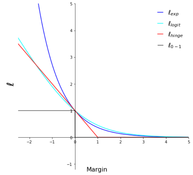
Loss functions

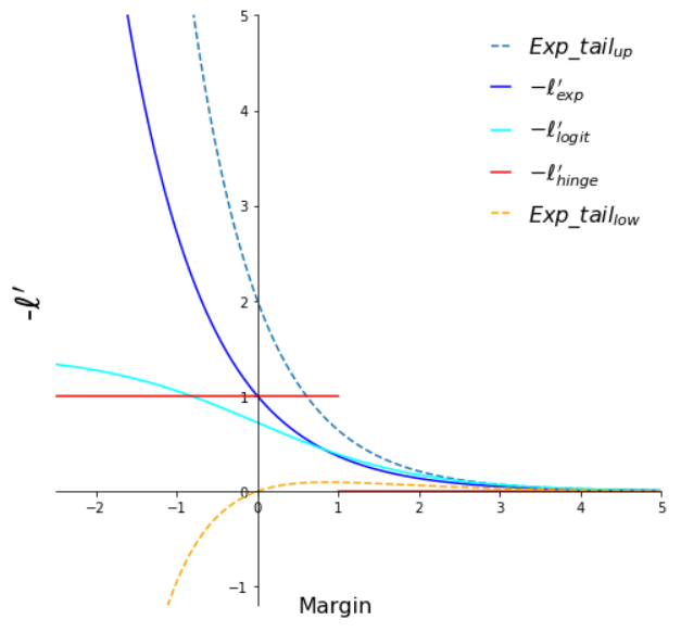
Negative derivatives of the loss functions

Illustration of tight exponential tail property for different common loss functions. We can see that both exponential and logistic loss functions have a tight exponential tail. The hinge loss and 0-1 loss functions have been displayed for reference only.

We consider the following classification problem:

\[\min_{w\in \R^d} \LL(w) = \min_{w\in \R^d} \sum_{i=1}^{n}\ell(y_i w^T x_i)\]

where $\forall i \in [\![ 1, n]\!], (x_i, y_i) \in \R^d\times\{-1,1\}$ and $\ell:\R \mapsto \R^*_+$ is a surrogate loss function of the $0$-$1$ loss.

We will study the behavior of the solution found by gradient descent using a fixed learning rate $\eta$:

\[w_{t+1} = w_{t} - \eta \nabla \LL(w_t) = w_{t} - \eta \sum_{i=1}^{n}\ell'(y_i w_t^T x_i)y_i x_i\]

Lemma 15. Let $\D = \{(x_i, y_i)\}_{i=1}^{n}$ be a linearly separable dataset where $\forall i \in [\![ 1, n]\!], (x_i, y_i) \in \R^d\times\{-1,1\}$ and $\ell:\R \mapsto \R^*_+$ a loss function under assumptions 1 and 2. Let $w_t$ be the iterates of gradient descent using learning rate $0<\eta<\frac{2}{\beta\sigma^2_{max}(X)}$ and any starting point $w_0$. Then we have:

$\lim_{t \xrightarrow{}\infty}\LL(w_t)=0$,
$\lim_{t \xrightarrow{}\infty}\norm{w_t}=\infty$,
$\forall i: \ \ \lim_{t \xrightarrow{}\infty} y_iw_t^Tx_i=\infty$,

Proof. As mentioned we use the exponential loss function: $\ell:u \mapsto e^{-u}$, which.
Since $\D$ is linearly separable, $\exists w_*$ such that $w_*^T x_i > 0, \forall i$. Then for $w \in \R^d$:
\[w_*^T\nabla \LL(w) = \sum_{i=1}^{n} \underbrace{-exp(-y_i w^T x_i)}_{<0} \underbrace{y_i w_*^T x_i}_{>0} < 0.\]
Therefore there is no finite critical points $w$, for which $\nabla \LL(w)=0$. But gradient descent on a smooth loss with an appropriate learning rate is always guaranteed to converge to a critical point : in other words $\nabla \LL(w_t)\xrightarrow{}0$. This necessarily implies that $\norm{w_t}\xrightarrow{}\infty$, which is (2). It also implies that $\exists t_0$ s.t, $\forall t>t_0, \forall i: y_i w_t^T x_i>0$ in order to make the exponential term converge to zero, this is (3). But in that case, we also have $\LL(w_t)\xrightarrow{}0$, which is (1). ◻

The norm of the previous solution diverges, but we can normalize it to have norm 1.

Theorem 16. Let $\D = \{(x_i, y_i)\}_{i=1}^{n}$ be a linearly separable dataset where $\forall i \in [\![ 1, n]\!], (x_i, y_i) \in \R^d\times\{-1,1\}$ and $\ell:\R \mapsto \R^*_+$ a loss function with under assumptions 1, 2 and 3. Let $w_t$ be the iterates of gradient descent using a learning rate $\eta$ such that $0<\eta<\frac{2}{\beta\sigma^2_{max}(X)}$ and any starting point $w_0$. Then we have:

\[\lim_{t \xrightarrow{}\infty}\frac{w_t}{\norm{w_t}}=\frac{w_{svm}}{\norm{w_{svm}}}\]

where $w_{svm}$ is the solution to the hard margin SVM:

$w_{svm} = \argmin_{w\in\R^d}\norm{w}^2\ \ s.t.\ \ y_i w^T x_i\geq 1, \forall i.$

Proof sketch. We will just give the main ideas behind the proof of this theorem using the exponential loss function. We will furthermore assume that $\frac{w_t}{\norm{w_t}}$ converges to some limit $w_{\infty}$. For a detailed proof and in the more general case of the loss function having properties 1 to 3 please refer to Soudry et al. (2018).

By Lemma 15 we have $\forall i:\ \lim_{t \xrightarrow{}\infty} y_iw_t^Tx_i=\infty$. As $\frac{w_t}{\norm{w_t}}$ converges to $w_{\infty}$ we can write $w_t = g(t)w_{\infty}+\rho(t)$ such that $g(t) \xrightarrow{}\infty$, $\forall i:\ y_iw^T_{\infty}x_i >0$ and $\ \lim_{t \xrightarrow{}\infty} \frac{\rho(t)}{g(t)}=0$. The gradient can then be written as:
\[\label{eq:neg_grad} - \nabla \LL(w_t) = \sum_{i=1}^{n} e^{-y_iw_t^Tx_i}x_i = \sum_{i=1}^{n} e^{-g(t)y_iw_{\infty}^Tx_i}\ e^{-y_i\rho(t)^Tx_i}x_i\]
We can see that as $g(t) \xrightarrow{}\infty$ only the samples with the largest exponents in the sum of the right-hand side of the last equation will contribute to the gradient. The exponents are maximized for $i \in \mathcal S = argmin_i\ y_iw_{\infty}^Tx_i$ which correspond to the samples minimizing the margin: i.e. the support vectors $X_S = \{x_i, i \in \mathcal S\}$. The negative gradient $- \nabla \LL(w_t)$ would then asymptotically become a non-negative linear combination of support vectors and because $\norm{w_t}\xrightarrow{}\infty$ (by Lemma 15) the first gradient steps will be negligible, and the limit $w_{\infty}$ will get closer and closer to a non-negative linear combination of support vectors and so will its scaled version $\hat w = w_{\infty}/\min_i y_iw_{\infty}^Tx_i$ (the scaling is done to make the margin of the support vectors equal to 1). We can therefore write:
\[\hat w = \sum_{i=1}^n \alpha_ix_i\quad with\ \left\{ \begin{array}{ll} \alpha_ix_i\geq 0 \ and\ y_i\hat w^T x_i=1\ if\ i\in \mathcal S\\ \alpha_ix_i= 0 \ and\ y_i\hat w^T x_i>1\ if\ i\notin \mathcal S \end{array} \right.\]
We can recognize the KKT conditions for the hard margin SVM problem (see Bishop (2006) Chapter 7, Section 7.1) and conclude that $\hat w = w_{svm}$. Then $\frac{w_{\infty}}{\norm{w_{\infty}}}=\frac{w_{svm}}{\norm{w_{svm}}}$. ○

In the proof of Lemma 15 we have seen that $\LL(w_t)\xrightarrow{}0$. That means that gradient descent converges to a global minimum.

Gradient descent has been suspected to induce a bias towards simple solutions, not only in these linear settings, but in deep learning as well, greatly improving generalization performance. It would explain the double descent behavior of deep learning architectures, and recent works such as Gissin et al. (2019) have been studying the learning dynamics in more complex settings.

In the next blog post we will explore two simple models for wich we can analyticaly prove the double descent phenomenon.